Benchmarks

The following benchmarks were run on a MacBook Pro laptop with an Apple M4 Max chip.

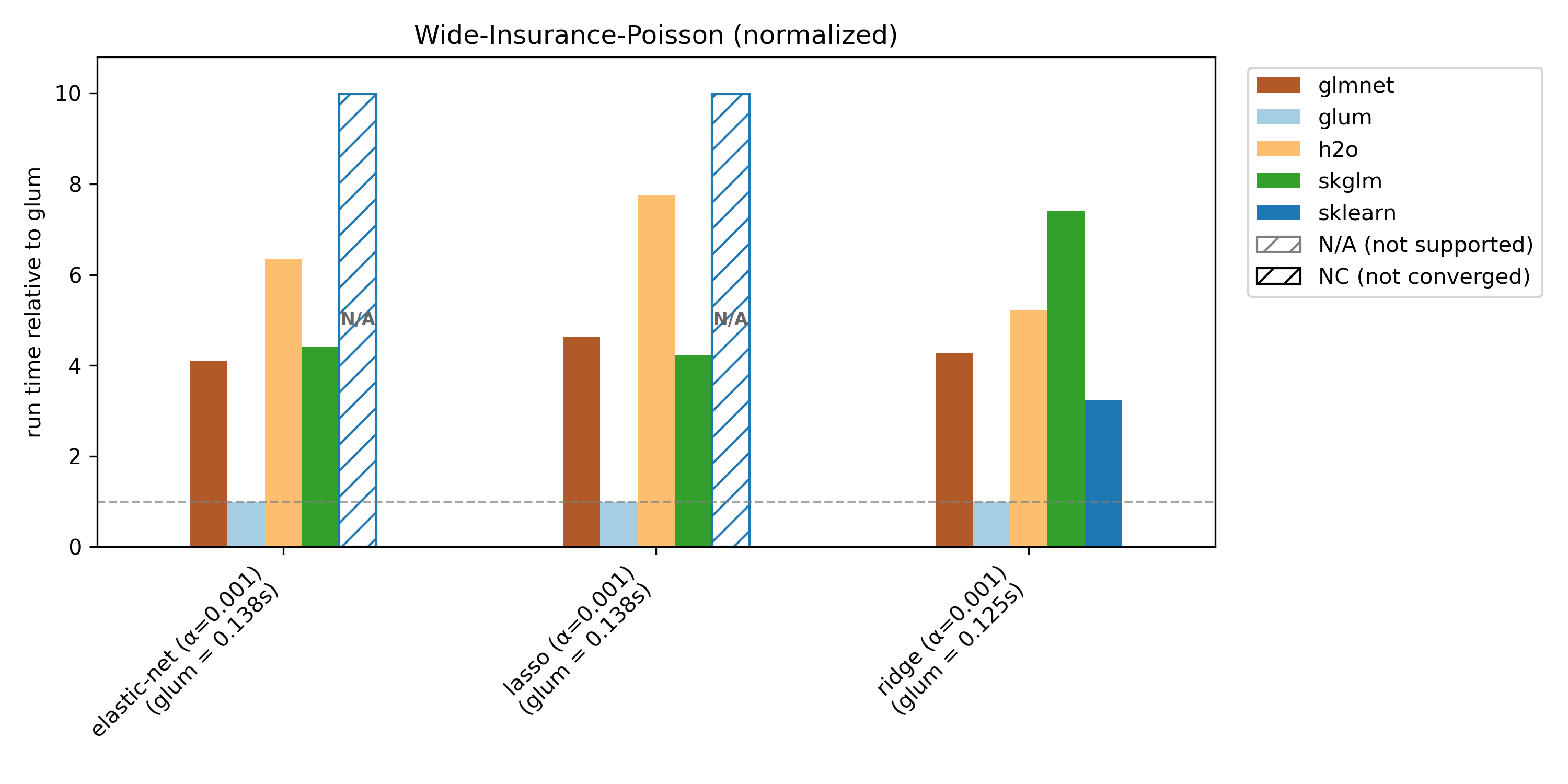
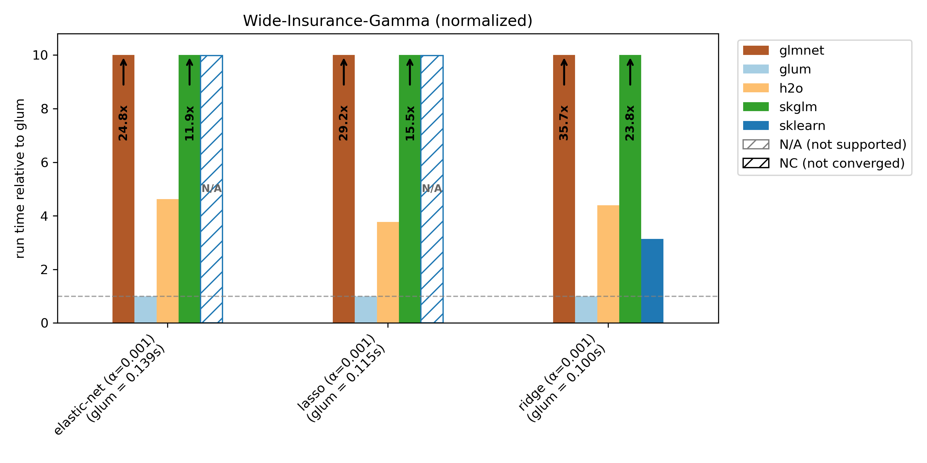
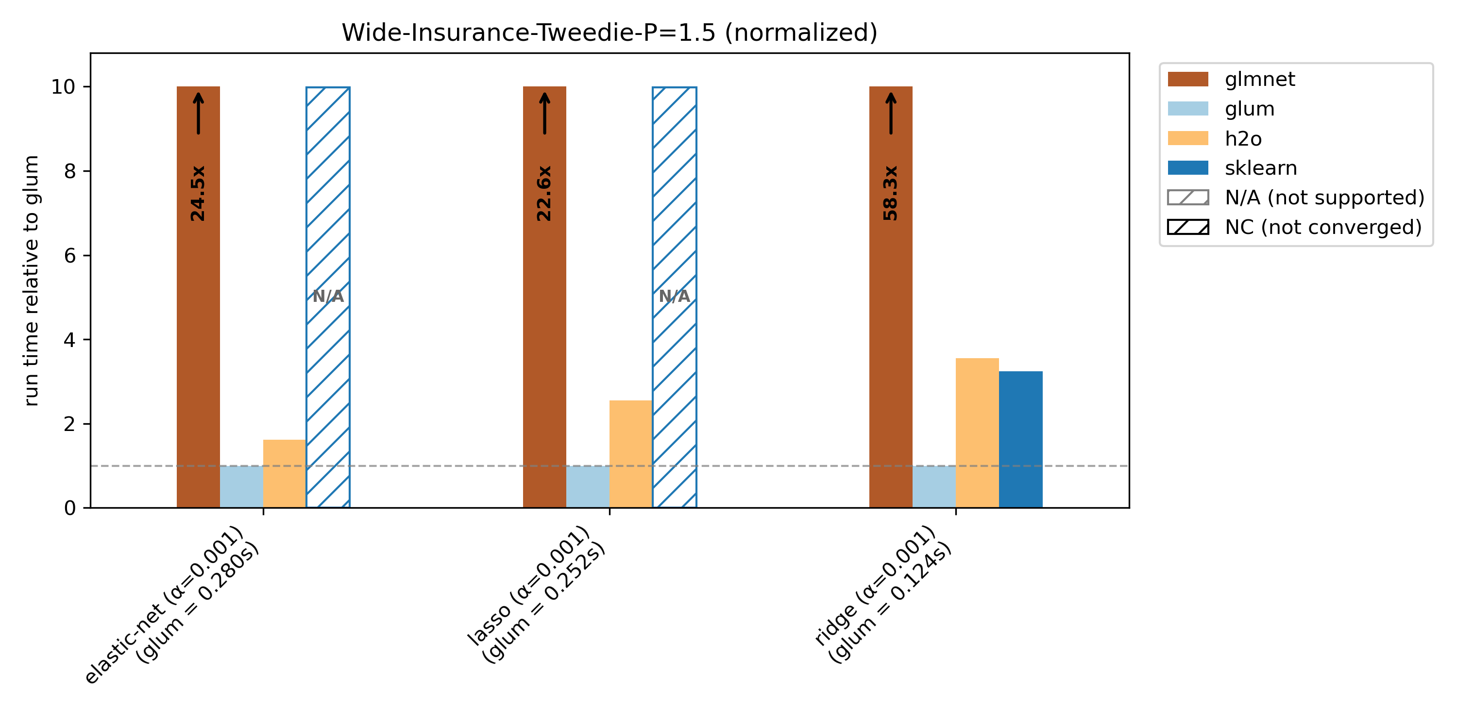
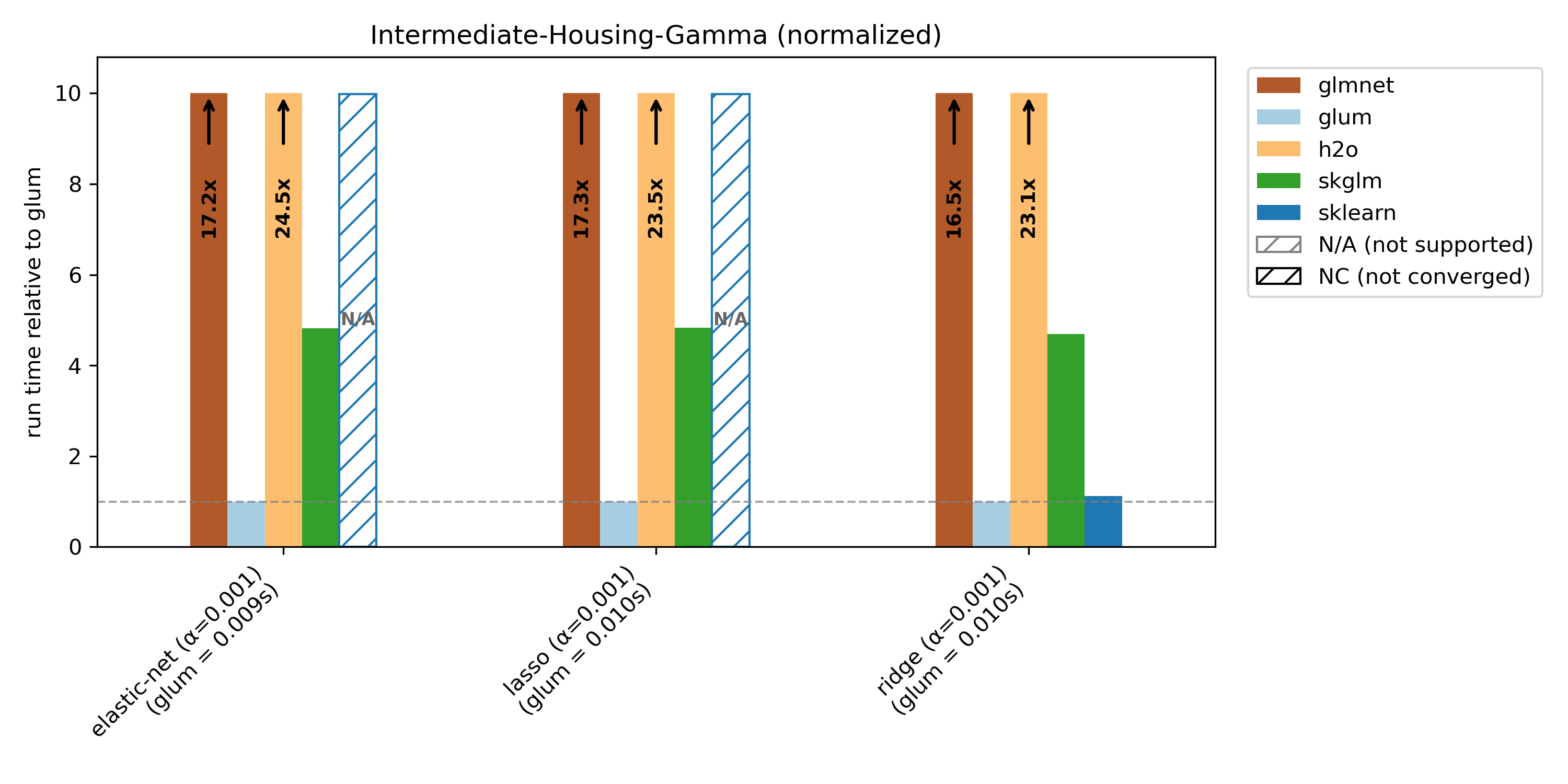
Each plot title indicates the dataset and distribution used. For example, “Wide-Insurance-Gamma” refers to the wide-insurance dataset fit with a gamma distribution. Further information about the datasets can be found at the end of the document.

For each dataset/distribution pair, we benchmark three regularization types:

• Elastic net (l1_ratio=0.5): elastic-net

• Ridge (l1_ratio=0.0): ridge

• Lasso (l1_ratio=1.0): lasso

We extract target variables and benchmark them under typical distributions (for example, insurance claim counts using Poisson models).

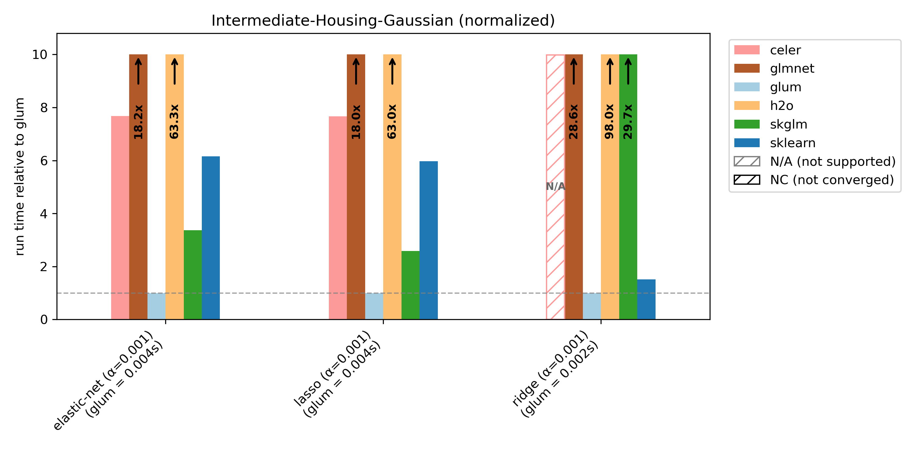
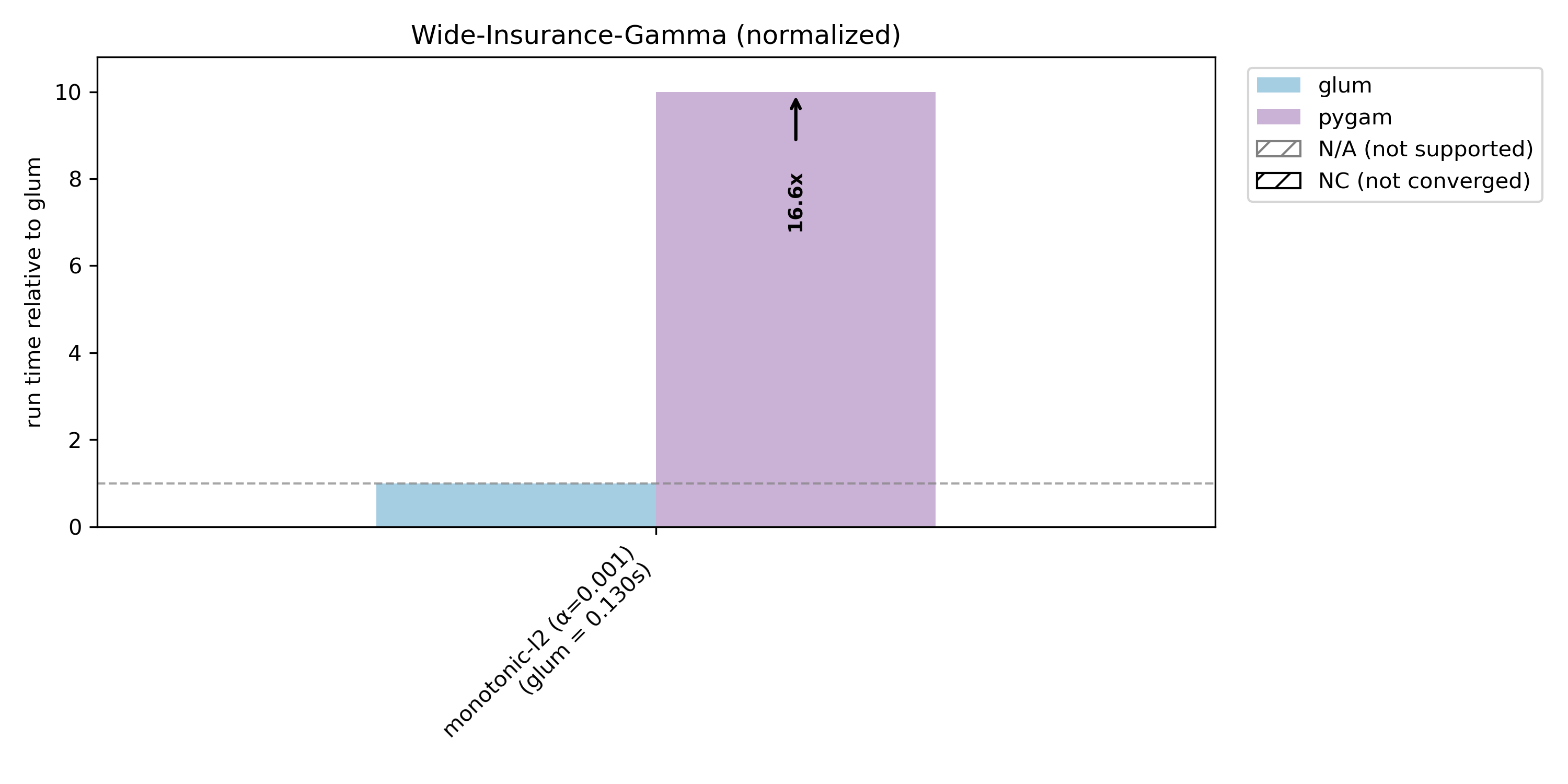
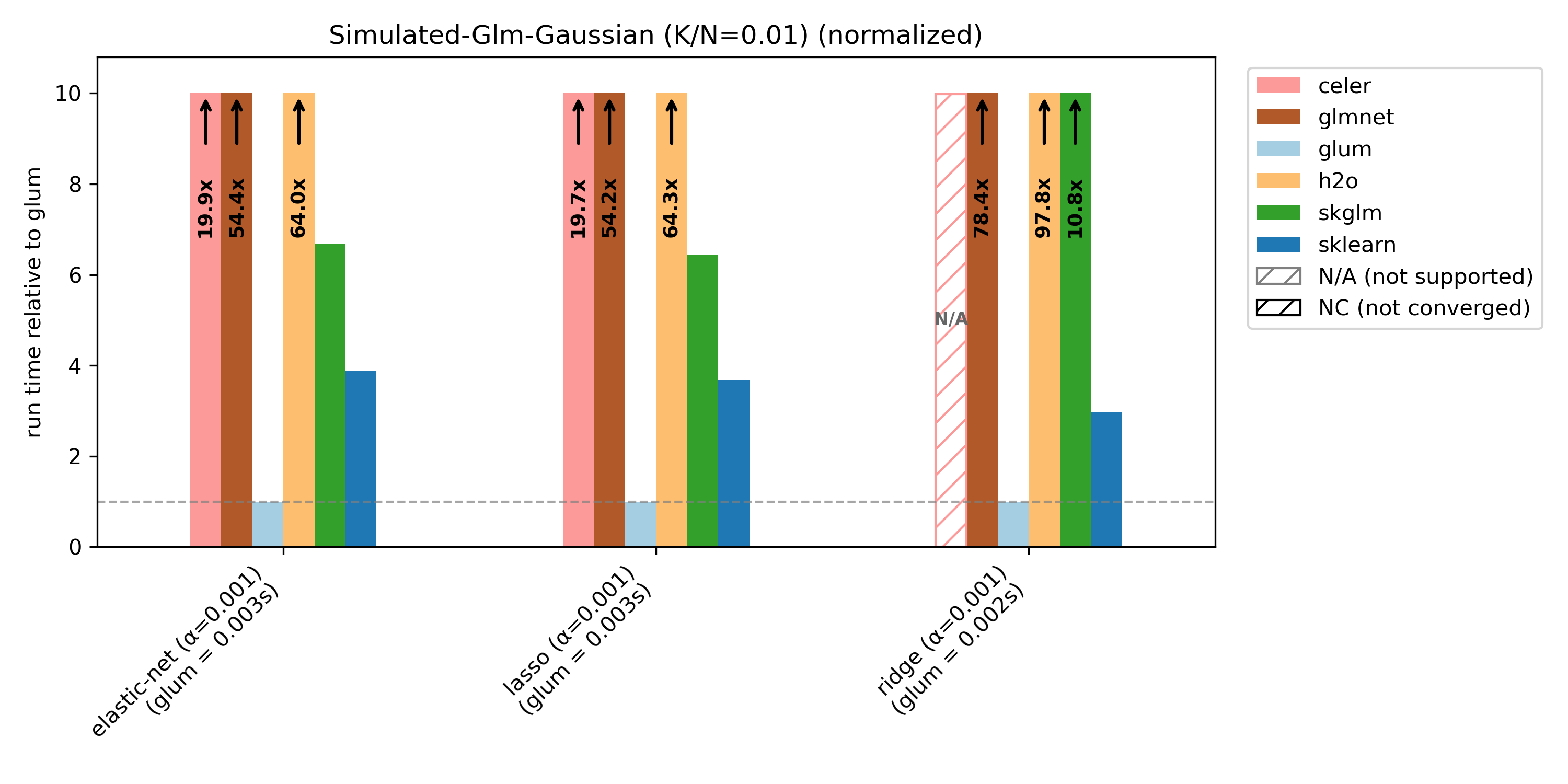
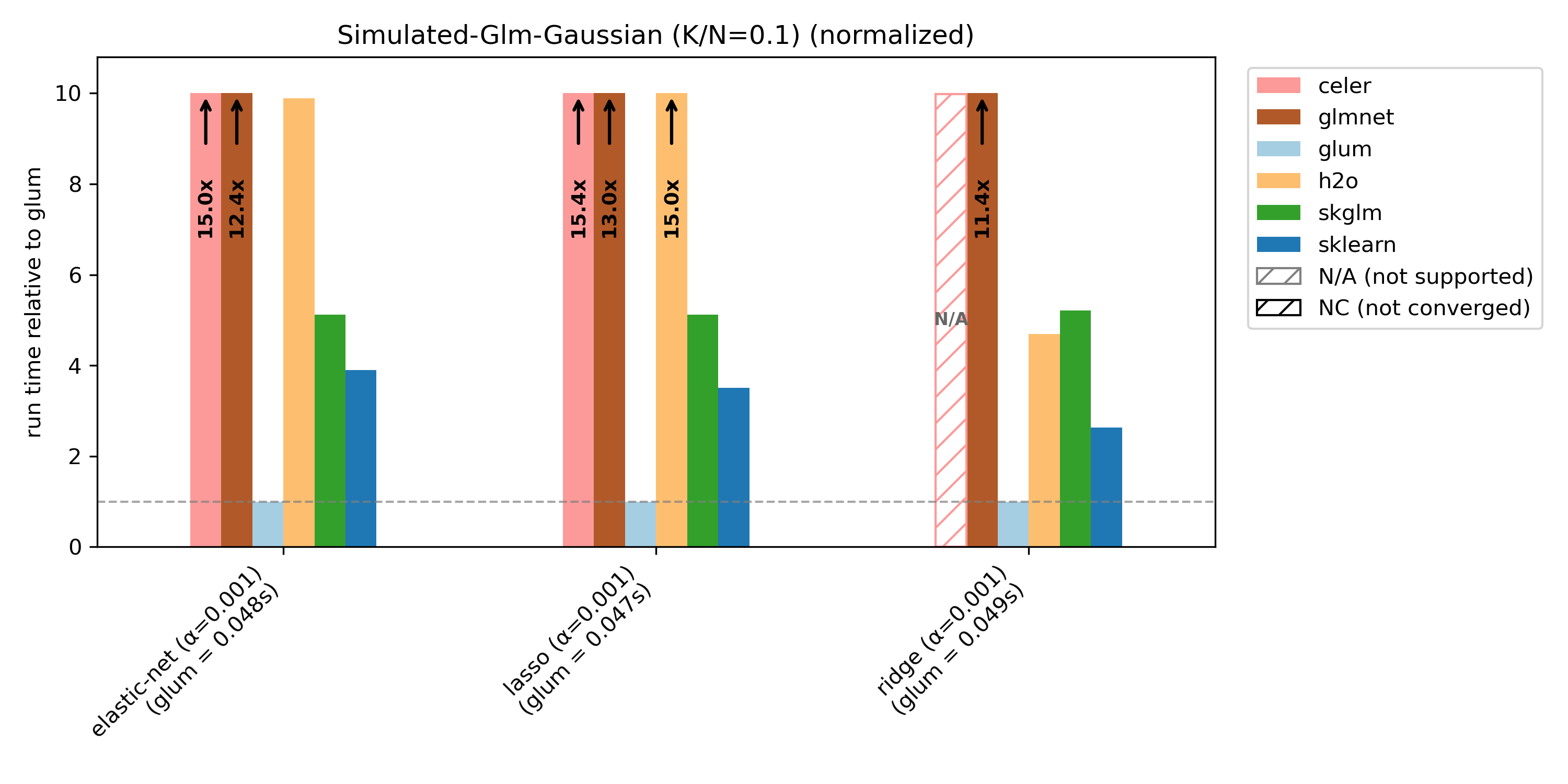
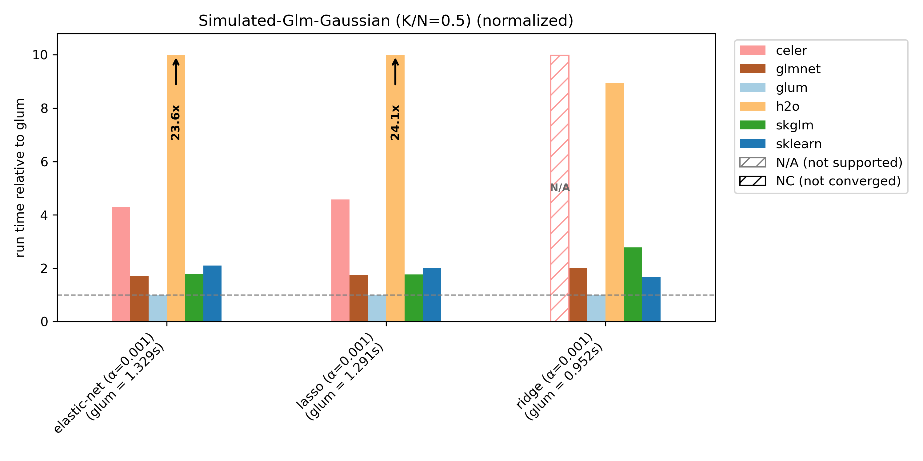
Runtime plots are reported relative to glum: for each benchmark case, glum’s runtime is normalized to 1.0 and other libraries’ runtimes are scaled accordingly. If a bar exceeds the plotting range, the exact runtime is printed on the bar and an arrow indicates truncation.

We compare glum against sklearn, skglm, glmnet, h2o and celer. As some libraries do not support all benchmark cases, these combinations are shown as N/A (not supported). If a library does not converge (either it reaches max_iter or exceeds the 100s timeout), it is shown as NC (not converged) at the maximum bar height.

glum was designed for settings with N >> K —that is, many more observations than predictors, apart from high-cardinality categorical features. This regime is well illustrated by the wide-insurance benchmark. For insurance data, we evaluate gamma, Poisson, and Tweedie distributions.

To showcase glum’s performance on another dataset, we also report results for intermediate-housing, which has N >> K and only numerical (no categorical) features. For this dataset, we benchmark gamma and Gaussian distributions.

glum also supports monotonic constraints on spline and ordered categorical terms, benchmarked here against pygam on the wide-insurance dataset with a gamma distribution.

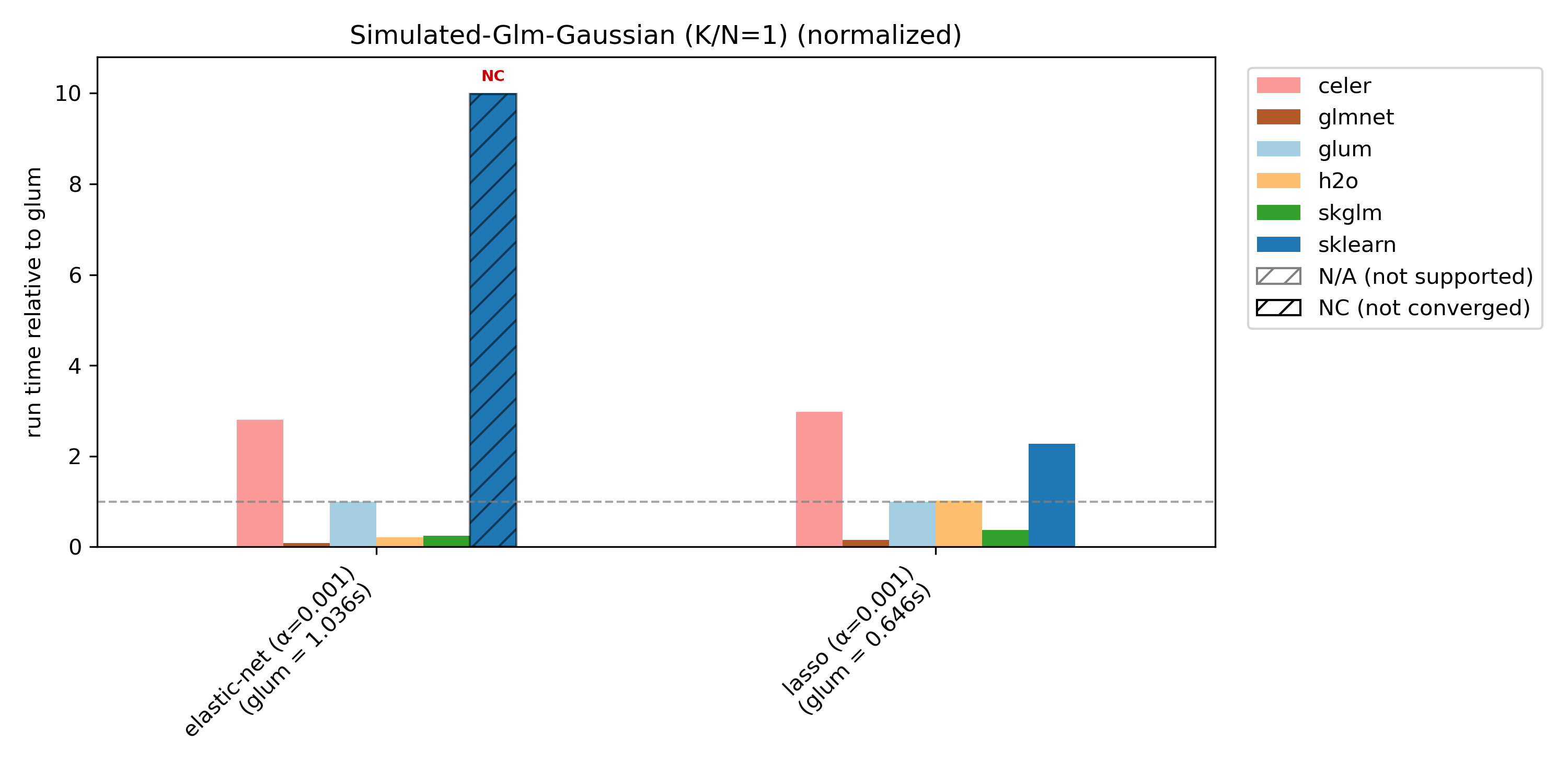
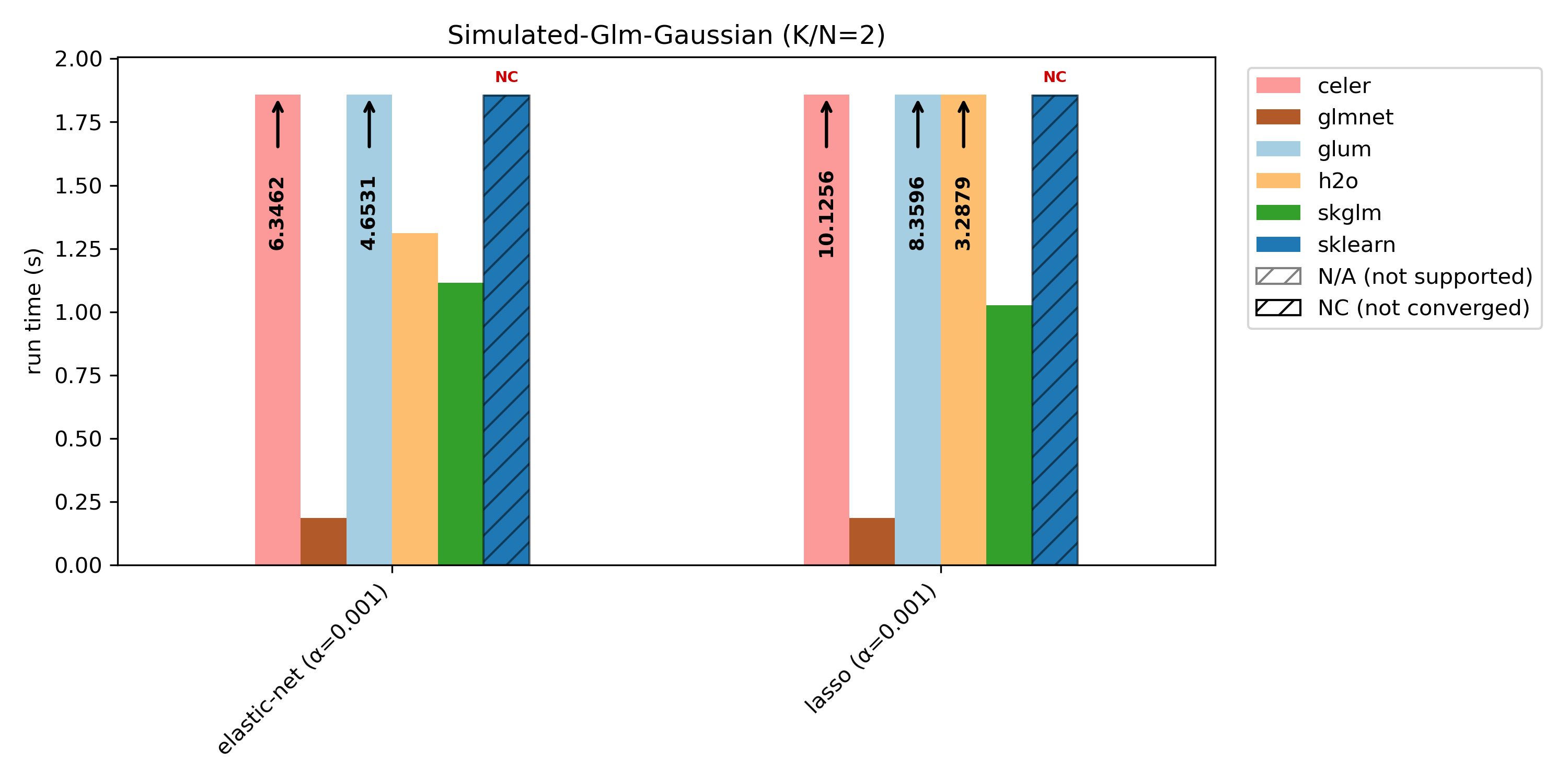
glum is primarily optimized for N >> K settings, and is not tuned for N ~ K or N < K. This is illustrated by the simulated benchmark with varying K/N ratios: glum performs best when N >> K, and relative performance decreases as K/N increases.

For K/N = 2, we include an unnormalized runtime plot, because in the normalized version the glmnet bar becomes too small to read clearly.

In the following table more information about the used datasets can be found. After filtering for ClaimAmountCut > 0 in the “Wide-Insurance-Gamma” dataset, only about 25,000 rows are left. We, therefore, artificially increase the dataset by sampling with replacement and adding noise. The filter is also why the number of columns after one-hot-encoding is smaller compared to the other distributions on this dataset because some category levels only exist in the dropped rows.

For simulated-glm we reduce N from 10 000 to 1 000 for K/N = 1 and K/N = 2 in order to speed things up (with N = 10 000 nearly no library converges within the 100s limit).

Dataset Overview

(Dataset, Distribution)	(N, K)	Cat. Columns	Num. Columns	Columns (OHE)	Source
(wide-insurance, poisson), (wide-insurance, tweedie)	(600 000, 9)	8	1	322	freMTPL2 + feature engineering/preprocessing
(wide-insurance, gamma)	(600 000, 9)	8	1	256	freMTPL2 + feature engineering/preprocessing
(intermediate-housing, poisson), (intermediate-housing, gamma)	(21 613, 10)	0	10	10	house_sales + feature engineering/preprocessing
(simulated-glm, gaussian) with K/N = 0.01	(10 000, 100)	0	100	100	simulated
(simulated-glm, gaussian) with K/N = 0.1	(10 000, 1 000)	0	1 000	1 000	simulated
(simulated-glm, gaussian) with K/N = 0.5	(10 000, 5 000)	0	5 000	5 000	simulated
(simulated-glm, gaussian) with K/N = 1	(1 000, 1 000)	0	1 000	1 000	simulated
(simulated-glm, gaussian) with K/N = 2	(1 000, 2 000)	0	2 000	2 000	simulated